Welcome to CBMOS’ documentation!¶

CBMOS is a Python framework for the numerical analysis of center-based models. It focuses on flexibility and ease of use and is capable of simulating up to a few thousand cells within a few seconds, or even up to 10,000 cells if GPU support is available. CBMOS shines best for exploratory tasks and prototyping, for instance when one wants to compare different sets of parameters or solvers. At the moment, it implements most popular force functions, a few first and second-order explicit solvers, and even one implicit solver. The following sections describe how to run a simple simulation and illustrate what kind of convergence studies can be performed with this package.

Getting Started¶

Initial condition¶

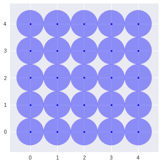
Setting up the initial condition of a simulation is very simple, all you need is create a list of cell objects. In this example we set up a Cartesian grid of 25 cells. Each cell will immediately divides after the simulation starts. This behavior is defined by the list of CellDivisionEvent objects. We then plot the current cell configuration using the basic plotting function provided in the utils module.

import numpy as np
import matplotlib.pyplot as plt

import cbmos
import cbmos.force_functions as ff
import cbmos.solvers.euler_forward as ef
import cbmos.cell as cl
import cbmos.utils as utils
import cbmos.events as events

n_x = 5
n_y = 5
coordinates = utils.generate_cartesian_coordinates(n_x, n_y)

sheet = [
    cl.ProliferatingCell(
        i, # Cell ID, must be unique to each cell
        [x,y], # Initial coordinates
        -6.0, # Birthtime, in this case 6 hours before the simulation starts
        True, # Whether or not the cell is proliferating
        lambda t: 6 + t # Function generating the next division time
    )
    for i, (x, y) in enumerate(coordinates)
]

event_list = [
    events.CellDivisionEvent(cell)
    for cell in sheet
]

utils.plot_2d_population(sheet)

Simulation¶

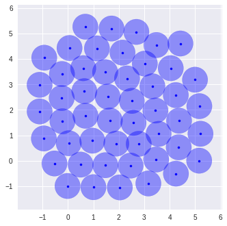
In this simulation, we use the Gls force and the Euler forward solver. The force function’s parameters are given to the simulate function as a dictionary. Parameters can also be passed to the solver in the same way. This function returns a tuple containing the time points and a list of cells for each of these time points. If needed a detailed log of the division events can be displayed by setting the log level to debug.

# Initialize model
model = cbmos.CBModel(ff.Gls(), ef.solve_ivp, dimension=2)

dt = 0.01
t_data = np.arange(0, 4, dt)

t_data, history = model.simulate(
    sheet, # Initial cell configuration
    t_data, # Times at which the history is saved
    {"mu": 5.70, "s": 1.0, "rA": 1.5}, # Force parameters
    {'dt': dt}, # Solver parameters
    event_list=event_list
)

utils.plot_2d_population(history[-1])

Exploring Convergence¶

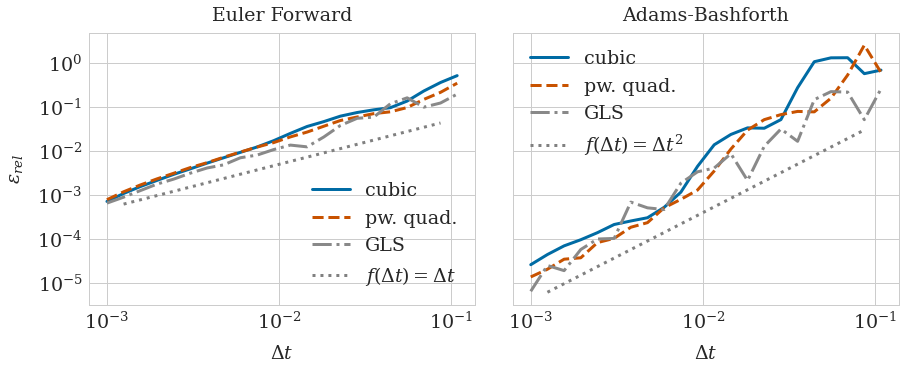
CBMOS is aimed at performing numerical studies of Center-Based overlapping Spheres Models. In this section, we present a minimal example to study the convergence of the Euler forward and Adams-Bashforth methods for a few non-proliferating cells and for three of the most popular force functions (namely GLS, Cubic and Piecewise Quadratic) can be studied.

Setup¶

After importing relevant modules, we set up the simulation parameters as well as all three models (one per force function). Each model takes three parameters: the force function to be used, the solver, and the dimension of the model (usually 2 or 3). For this simple example, we will use Euler Forward for all models.

import cbmos
import cbmos.force_functions as ff
import cbmos.solvers.euler_forward as ef
import cbmos.solvers.adams_bashforth as ab
import cbmos.cell as cl

import numpy as np
import scipy.interpolate as sci

# Simulation parameters
s = 1.0    # rest length
tf = 4.0  # final time
rA = 1.5   # maximum interaction distance
dim = 2

forces = {
    'cubic':ff.Cubic(),
    'pw. quad.':ff.PiecewisePolynomial(),
    'GLS': ff.Gls()
}

solvers = {
    'EF': ef.solve_ivp,
    'AB': ab.solve_ivp,
}

models = {
        solver_name: {
            force_name: cbmos.CBModel(
                             force,
                             solver,
                             dim,
                         )
            for force_name, force in forces.items()}
    for solver_name, solver in solvers.items()
}

Initial Conditions¶

Then, we create a list a cells using a list of (x, y) coordinates. Each cell takes at least 2 parameters: a (unique) id, and some coordinates. Optional parameters can be used to define if and when each cell should proliferate. In this example, and for the sake of simplicity, we will only not use proliferation. Cells are set to be at 30% of their rest lenght. Once the simulation is launched, the cells will push each other and relax to a new configuration.

import numpy.random as npr

n_x = 5
n_y = 5
compactness = 0.3

initial_sheet = [
    cl.Cell(i, [compactness*x, compactness*y])
    for i, (x, y) in enumerate(
        [(x, y) for x in range(n_x) for y in range(n_y)])
]

Model Parameters¶

The parameters of each force function can be set with a dictionnary containing all keywords argument to be passed to the force functions. In this case, the parameters are taken from [1], where they were set so that the relaxation time between the cells is one hour.

params_cubic = {
    "mu": 5.70,
    "s": s,
    "rA": rA,
}

muR = 9.1
ratio = 0.21
params_poly = {
    'muA': ratio*muR,
    'muR': muR,
    'rA': rA,
    'rR': 1.0/(1.0-np.sqrt(ratio)/3.0),
    'n': 1.0,
    'p': 1.0,
}

mu_gls=1.95
params_gls = {
    'mu': mu_gls,
    'a':-2*np.log(0.002/mu_gls),
}

params = {
    'cubic': params_cubic,
    'pw. quad.': params_poly,
    'GLS': params_gls,
}

Reference Solutions¶

Here we compute the reference solutions for each force functions, using fine timesteps. The simulate function takes the inital configuration of the cell sheet, the time span over which to perform the simulation, the parameters to be used for the force functions, and the parameters to pass to the numerical solver.

In this case, since we are interested in measuring the error at the timesteps used by the solver, we set raw_t to True. Otherwise, the simulator would interpolate the position of the cells at the times specified in t_data_ref. The exact timesteps used by the solver are then returned along the history, containing the configurations of the cells at each time point. In this example we convert this history into a numpy array for efficiency.

dt_ref = 0.0005

N_ref = int(1/dt_ref*tf)+1
t_data_ref = np.arange(0, tf, dt_ref)

ref_traj = {}
for solver in solvers:
    for force in forces:
        t_data_ref, history = models[solver][force].simulate(
            initial_sheet,
            t_data_ref,
            params[force],
            {'dt': dt_ref},
            raw_t=True,
        )

        ref_traj.setdefault(solver, {})[force] = np.array(
            [
                [cell.position for cell in cell_list]
                for cell_list in history
            ]
        ) # (N_ref, n_cells, dim)

Error computation¶

We now compute the error between the reference solution and solutions computed with coarser timesteps.

dt_values = np.array([0.001*1.25**n for n in range(0, 22)])

sol = {}
for dt in dt_values:
    N = int(1/dt*tf) + 1
    t_data = np.arange(0, tf, dt)

    for solver in solvers:
        for force in forces:
            t_data_sol, history = models[solver][force].simulate(
                initial_sheet,
                t_data,
                params[force],
                {'dt': dt},
                raw_t=True,
            )

            traj = np.array([
                [cell.position for cell in cell_list]
                for cell_list in history
            ]) # (N, n_cells, dim)
            interp = sci.interp1d(
                t_data_sol, traj,
                axis=0,
                bounds_error=False,
                fill_value=tuple(traj[[0, -1], :, :])
            )(t_data_ref[:])
            error = (
                np.linalg.norm(
                    interp - ref_traj[solver][force],
                    axis=0)
                /np.linalg.norm(
                    ref_traj[solver][force],
                    axis=0)
            ).mean(axis=0)

            sol.setdefault(solver, {})\
                .setdefault(force, [])\
                .append(error)

Convergence Plot¶

import matplotlib.pyplot as plt

plt.style.use('seaborn-whitegrid')
plt.style.use('tableau-colorblind10')
params = {'legend.fontsize': 'xx-large',
          'figure.figsize': (6.75, 5),
          'lines.linewidth': 3.0,
         'axes.labelsize': 'xx-large',
         'axes.titlesize':'xx-large',
         'xtick.labelsize':'xx-large',
         'ytick.labelsize':'xx-large',
          'legend.fontsize': 'xx-large',
         'font.size': 11,
          'font.family': 'serif',
          "mathtext.fontset": "dejavuserif",
         'axes.titlepad': 12,
        'axes.labelpad': 12}
plt.rcParams.update(params)

defcolors = plt.rcParams['axes.prop_cycle'].by_key()['color']
colors = {
    'cubic': defcolors[0],
    'pw. quad.': defcolors[5],
    'GLS': defcolors[6],
}
linestyles = {
    'cubic': '-',
    'pw. quad.': '--',
    'GLS': '-.',
}

fig, ax = plt.subplots(
    1, 2,
    figsize=(14.5, 5),
    sharey=True,
    gridspec_kw={'wspace': 0.1},
)

for i, solver in enumerate(solvers):
    for force in forces:
        ax[i].loglog(
            dt_values,
            np.sum(np.array(sol[solver][force]), axis=1),
            label=force,
            color=colors[force],
            linestyle=linestyles[force]
        )

    ax[i].set_xlabel('$\Delta t$')

ax[0].set_title('Euler Forward')
ax[1].set_title('Adams-Bashforth')

ax[0].loglog(dt_values[1:-1], dt_values[1:-1]*0.5, ':',
           label='$f(\Delta t)= \Delta t$', color='grey')
ax[1].loglog(dt_values[1:-1], dt_values[1:-1]**2*4, ':',
           label='$f(\Delta t)= \Delta t^2$', color='grey')


ax[0].set_ylabel('$\epsilon_{rel}$')
ax[0].legend(loc=0)
ax[1].legend(loc=0)

plt.show()

References¶

Mathias, S., Coulier, A., Bouchnita, A., & Hellander, A. (2020). Impact of force function formulations on the numerical simulation of centre-based models. Bulletin of Mathematical Biology, 82(10), 1-43.

Implementing your own events¶

Although the events we provide in this package are relatively limited, CBMOS is designed to be flexible enough to use any event you wish to implement.

New event can easily be implemented by deriving the abstract Event class and overriding the __init__ and apply methods. As mentionned in Event class’ documentation, the only requirement is that the new subclass possesses an attribute tau, which represents the time at which the event is triggered. The apply method takes an object of type CBModel as unique parameter. This object contains all the information about the current simulation and can be used to add, modify and remove cells.

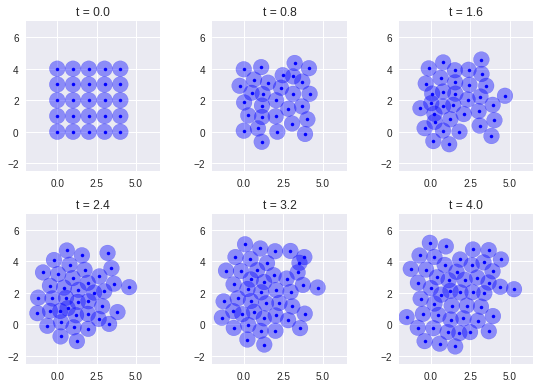
In this example, we implement two simple events:

GlobalDeathEvent selects one cell at random and removes it from the simulation.
GlobalDivisionEvent selects one cell at random and duplicates it.

Here, we set the simulation so that these events are triggered at regular intervals. This mimics other cell-based software, where the simulation is stopped at regular intervals to check if events have taken place.

Although cell division and cell death can be implemented in many different ways, depending of the complexity of the biological model. We hope these examples illustrate how CBMOS can handle such a variety of possibilities.

import numpy as np
import numpy.random as npr

npr.seed(0)

from cbmos.events import Event
from cbmos.cell import Cell

class GlobalDeathEvent(Event):
    def __init__(self, tau):
        self.tau = tau

    def apply(self, cbmodel):
        target_cell = npr.choice(cbmodel.cell_list)
        del cbmodel.cell_list[npr.randint(len(cbmodel.cell_list))]

class GlobalDivisionEvent(Event):
    def __init__(self, tau):
        self.tau = tau

    def apply(self, cbmodel):
        target_cell = npr.choice(cbmodel.cell_list)

        division_direction = self.get_division_direction(cbmodel)
        updated_position_parent = target_cell.position \
            - 0.5 * cbmodel.separation * division_direction
        position_daughter = target_cell.position \
            + 0.5 * cbmodel.separation * division_direction

        daughter_cell = Cell(cbmodel.next_cell_index, position_daughter)
        cbmodel.next_cell_index += 1
        cbmodel.cell_list.append(daughter_cell)

        target_cell.position = updated_position_parent

    def get_division_direction(self, cbmodel):
        if cbmodel.dim == 1:
            division_direction = np.array([-1.0 + 2.0 * npr.randint(2)])

        elif cbmodel.dim == 2:
            random_angle = 2.0 * np.pi * npr.rand()
            division_direction = np.array([
                np.cos(random_angle),
                np.sin(random_angle)])

        elif cbmodel.dim == 3:
            u = npr.rand()
            v = npr.rand()
            random_azimuth_angle = 2 * np.pi * u
            random_zenith_angle = np.arccos(2 * v - 1)
            division_direction = np.array([
                np.cos(random_azimuth_angle) * np.sin(random_zenith_angle),
                np.sin(random_azimuth_angle) * np.sin(random_zenith_angle),
                np.cos(random_zenith_angle)])

        return division_direction

import numpy as np

import cbmos.cell as cl
import cbmos.utils as utils

T = 4
t_data = np.linspace(0, T, num=6)

n_x = 5
n_y = 5
coordinates = utils.generate_cartesian_coordinates(n_x, n_y)

sheet = [
    cl.Cell(
        i, # Cell ID, must be unique to each cell
        [x,y], # Initial coordinates
    )
    for i, (x, y) in enumerate(coordinates)
]

event_list = [
    GlobalDivisionEvent(tau)
    for tau in np.linspace(0, T, num=50)
] + [
    GlobalDeathEvent(tau)
    for tau in np.linspace(0, T, num=25)
]

import cbmos
import cbmos.force_functions as ff
import cbmos.solvers.euler_forward as ef

# Initialize model
model = cbmos.CBModel(ff.Gls(), ef.solve_ivp, dimension=2)

t_data, history = model.simulate(
    sheet, # Initial cell configuration
    t_data, # Times at which the history is saved
    {"mu": 5.70, "s": 1.0, "rA": 1.5}, # Force parameters
    {'dt': 0.01}, # Solver parameters
    event_list=event_list,
    raw_t=False,
)

import matplotlib.pyplot as plt

color = 'blue'

fig, ax = plt.subplots(2, 3)
for i, cells in enumerate(history):
    for cell in cells:
        ax[i//3, i%3].add_patch(plt.Circle(cell.position, 0.5, color=color, alpha=0.4))
        ax[i//3, i%3].plot(cell.position[0], cell.position[1], '.', color=color)
        ax[i//3, i%3].set_aspect('equal')
        ax[i//3, i%3].set_xlim(-2, 6.5)
        ax[i//3, i%3].set_ylim(-2.5, 7)
        ax[i//3, i%3].set_title(f"t = {t_data[i]:.1f}")

fig.tight_layout()

cbmos¶

cbmos package